
As a technical SEO, you might be diving into machine learning (ML) to understand how tools like Google’s Gemini process text. One foundational concept is subword tokenization—breaking words into smaller pieces called “tokens.” While tokens themselves are context-agnostic (they don’t consider surrounding words), they do carry an inherent bias: each token’s likelihood reflects how prominent that subword was in the training data. In other words, tokens that appeared frequently during training end up with higher scores, and this directly influences downstream ML models.
By using the following tool, you can inspect which subwords are common or rare, helping you anticipate how Google’s Gemini might treat certain tokens in content, prompts and search queries.
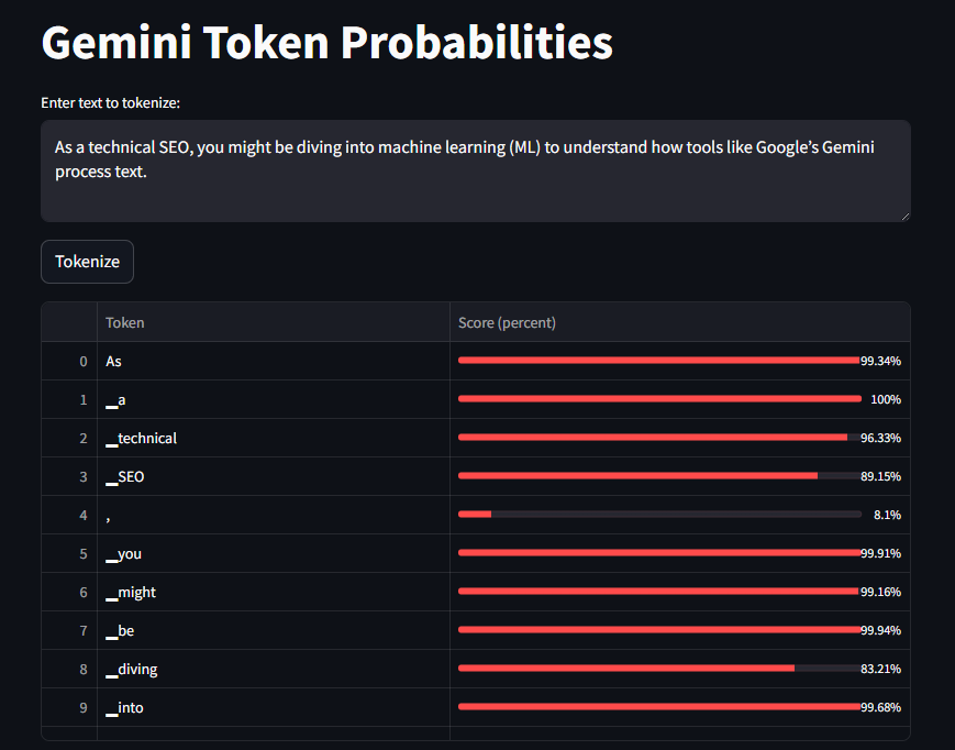
https://dejan.ai/tools/gemini-tokenizer
This tool is not a simulation. It uses Gemini’s actual trained SentencePiece model.
Background: Subword Tokenization and SentencePiece
Before diving into scores, it helps to recall why we use subword tokenization at all:
- Vocabulary Size vs. Coverage
- A simple “word-level” tokenizer might end up with millions of out-of-vocabulary (OOV) tokens, hurting model performance when it sees rare or new words.
- A pure “character-level” tokenizer avoids OOV but leads to longer input sequences, which can be inefficient.
- Subword Balance
- Subword tokenization (e.g., Byte-Pair Encoding, Unigram models) strikes a balance: common words remain intact as single tokens, while rare words are split into smaller subword pieces.
- This ensures that even a completely unseen word can be decomposed into known subwords (e.g., “quantumization” → “quant@@”, “um@@”, “ization”).
SentencePiece’s unigram approach proceeds roughly as follows:
- Candidate Extraction
- Given a large corpus, it extracts a large pool of possible subword candidates (up to hundreds of thousands).
- Unigram Model Training
- It fits a simple unigram language model over these candidates. Each candidate piece adopts a “score” (a log-probability) that indicates how likely that piece is to appear—under a generative assumption that tokens occur independently (hence “unigram”).
- Iterative Pruning
- Based on this initial scoring, SentencePiece prunes low-scoring/low-frequency pieces, retrains the unigram model, and repeats until it arrives at a target vocabulary size (e.g., 50 K tokens).
- The final set of pieces—plus their learned log-likelihood scores—constitute the tokenizer.
These learned log-likelihoods are the “raw scores” we’ll explore. In many applications (like our Streamlit demo), we normalize them across the entire vocabulary so that end users can see a “percentage-style” bar indicating each token’s relative importance during training.
What Do These Scores Really Represent?
It is tempting to read “log-likelihood” as simply “how often did this exact subword occur in the training data?” In reality, SentencePiece’s unigram training infers each piece’s probability by optimizing corpus reconstruction. Concretely:
- Not Raw Counts
- A raw count might say “‘ing’ appeared 1.2 million times.” But SentencePiece instead fits a probabilistic model:
[math]
\text{maximize } \prod_{w \in \text{corpus}} \sum_{\text{tokenizations } t \rightarrow w} \prod_{u \in t} P(u).
[/math]
During this optimization, each subword piece [math]u[/math] gets assigned a probability [math]P(u)[/math]. Taking the log yields the “log-likelihood” or “score” used internally.
- Log-Likelihood vs. Frequency
- Because it’s a log-probability, a piece with higher log-likelihood is both more frequent and more valuable for reconstructing many words in the corpus.
- Low-frequency fragments might be pruned away even if they appear occasionally, simply because including them adds complexity without significantly improving reconstruction accuracy.
- Global, Context-Agnostic
- Crucially, these scores do not depend on neighboring tokens (no left- or right-context). They reflect a piece’s overall importance to the tokenizer’s ability to model the entire training corpus—hence “unigram.”
Framing Scores as “Token Likelihood”
When presenting these scores to readers or end users, it’s helpful to describe them as a “likelihood of the token appearing in the training data”, with these caveats:
- Unigram-Model Likelihood
- Each piece’s bar represents its unigram-model log-likelihood, i.e., [math]\log P(u)[/math] for subword [math]u[/math]. You can say: “This is the likelihood that SentencePiece’s unigram learner associated with each subword based on how often (and how crucially) it appeared in the training corpus.”
- Normalization for Visualization
- Raw log-scores can be large negative values (e.g., [math]-6.12[/math], [math]-3.45[/math], [math]-9.88[/math]). To display them as a 0–100 % bar, you:
- Compute global minimum [math]\bigl(\min_{\text{all tokens}} \log P\bigr)[/math] and global maximum [math]\bigl(\max \log P\bigr)[/math].
- Linearly map each raw score into [math][0,1][/math]:
[math]
\text{Normalized}(u) = \frac{\log P(u) – \min \log P}{\max \log P – \min \log P}.
[/math]
Render “Normalized” as a percentage (0 % = least likely piece; 100 % = most likely piece).
Avoiding Misinterpretation
Because some readers might confuse this with “the probability a model would generate this token next,” emphasize:
“These are unnormalized log-probabilities from tokenizer training (unigram), not the conditional probabilities you’d get from a full language model.”
Framing as “Importance”
You can say, for instance:
> “A higher-scoring token was more central to reconstructing the training data and thus was retained in the final vocabulary.”
In other words, “importance during tokenizer training” and “likelihood of appearing” are two sides of the same coin under the unigram model.
Example Paragraph for the Article
Token Likelihood (Unigram Score).
Each subword piece in our SentencePiece-based Gemini tokenizer carries a unigram log-likelihood—a number learned during tokenizer training to maximize the model’s ability to reconstruct the corpus. Intuitively, tokens that appeared more frequently (or that helped reconstruct many different words) receive higher log-probabilities. In our visualization, we then linearly map these raw log-scores into a [math][0,1][/math] range and display them as percentages (0 % = lowest “importance,” 100 % = highest). Note that this is a global, context-agnostic measure: it does not depend on what comes before or after. Rather, it reflects how “likely” that piece was under the SentencePiece unigram model of the training data.
Interpreting “Token Likelihood” in Practice
- Common English Subwords Tend to Top the List
- Pieces like [math]“Ġthe”[/math] (where “Ġ” denotes a leading space) or [math]“ing”[/math] will typically have near-100 % bars, since they appear extremely often in running text.
- Rare fragments (e.g., [math]“Ġž̌̌”[/math] or very specialized technical tokens) end up with very low log-scores and thus display near-0 % bars.
- Vocabulary Pruning & Efficiency
- During training, lower-scoring candidates were likely pruned away to shrink the vocabulary. The final set of ~50 K tokens represents those pieces that best balanced coverage (capturing most words) with compactness.
- The bar plot visually underscores which pieces were essential (high bar) versus borderline cases (mid-to-low bar).
- Why “Likelihood of Appearing” Matters
- If you’re crafting a domain-specific dataset, you might compare your domain’s token frequencies against these precomputed scores to see which pieces may be underrepresented.
- For interactive demos (like our Streamlit interface), showing users these bars helps them understand which segments of their input text are “common” vs. “rare” from the tokenizer’s perspective.
Caveats and Common Pitfalls
- Not a Contextual Probability
Never say “this bar indicates the chance the next token will be X.” Instead, always clarify it’s a unigram score that’s context-independent. - Log-Probability ≠ Raw Count
If a token shows a “70 %” bar, that does not mean “it occurred in 70 % of all training sentences.” It means its log-probability was 70 % of the way between the worst and best log-scores in the entire vocabulary. - Normalization Dependent on Vocabulary
If you later retrain the tokenizer with a different size (e.g., 32 K vs. 50 K tokens), the raw min/max log-scores shift. Thus a “70 %” in a 32 K-token vocabulary is not numerically identical to a “70 %” in a 50 K-token vocabulary.
Putting It All Together: A Sample Section
#### Token Likelihoods in Action
When you type a sentence like “The quick brown fox jumps over the lazy dog”, our interface will break it into subword pieces such as:
[“ĠThe”, “Ġquick”, “Ġbrown”, “Ġfox”, “Ġjumps”, “Ġover”, “Ġthe”, “Ġlazy”, “Ġdog”]For each subword, we look up its learned unigram log-likelihood (e.g., [math]“Ġthe”[/math] might have [math]\log P = -2.1[/math], [math]“Ġquick”[/math] [math]\log P = -5.3[/math], [math]“Ġfox”[/math] [math]\log P = -6.2[/math]). After computing the global min and max over all ~50 K tokens, we map these values into [math][0,1][/math]. Suppose:
- min log-score = [math]-9.8[/math]
- max log-score = [math]-1.5[/math] Then for [math]“Ġthe”[/math]:
[math]
\text{Normalized} = \frac{-2.1 – (-9.8)}{-1.5 – (-9.8)} = \frac{7.7}{8.3} \approx 0.928 \,(\approx 92.8\%).
[/math]
For [math]“Ġfox”[/math]:
[math]
\text{Normalized} = \frac{-6.2 – (-9.8)}{-1.5 – (-9.8)} = \frac{3.6}{8.3} \approx 0.434 \,(\approx 43.4\%).
[/math]
Visually, [math]“Ġthe”[/math] will show a long, nearly full bar (indicating it was extremely common), while [math]“Ġfox”[/math] will be roughly halfway (moderately common).
Framing these SentencePiece scores as a “likelihood of the token appearing in the training data” is accurate when you emphasize:
- They are learned unigram log-likelihoods, not raw frequency counts.
- The values are context-agnostic—no dependence on surrounding tokens.
- We linearly normalize them into [math][0,1][/math] and display as percentages for intuitive visualization.
By clarifying these points in your article, readers will gain a clear understanding of why some subword pieces are deemed more “important,” how the normalization step works, and what these bars truly signify. This transparent framing helps set proper expectations and prevents misinterpretation: the bars represent global importance during tokenizer training, not “the probability that your model will output this next.”
Gemini 1.5 Pro Tokenizer: Vocabulary, Scores, and Internal Structure
Below is an in-depth look at the actual gemini-1.5-pro-002.spm.model file (a SentencePiece “unigram” tokenizer).
We’ll cover:
- Vocabulary Size and Special Tokens
- Score Distribution (Log-Likelihoods)
- Typical High- and Low-Scoring Pieces
- Internal Structure of the
.spm.modelFile
1. Vocabulary Size and Special Tokens
When you load gemini-1.5-pro-002.spm.model with SentencePieceProcessor (using sp.Load("…/gemini-1.5-pro-002.spm.model")), you discover:
- Total Pieces (“Vocabulary Size”)
sp.GetPieceSize() ➔ 256000In other words, this tokenizer defines 256000 distinct “subword” pieces.
- Dedicated Control & Special Tokens
Among these 256000 entries, there are about 506 pieces whose log-likelihood score is exactly 0.0. These include: <pad>(ID 0)- Unused placeholders like
<unused0>,<unused1>, …,<unused99> - Hex-notation codepoint tokens such as
<0x5E>,<0x6A>, etc. - Other control tokens (e.g. end-of-sentence, unknown, BOS/EOS markers, etc.) You can verify this by running in Python:
  zero_count = sum(1 for i in range(sp.GetPieceSize()) if sp.GetScore(i) == 0.0)
  # zero_count ➔ 506
Any piece with a score of 0.0 is reserved (not “learned” from the corpus) and typically used for padding, special markers, or placeholders.
2. Score Distribution (Log-Likelihoods)
Each subword piece u in a SentencePiece unigram model carries a log-likelihood \log P(u). In this particular .spm.model, the raw score range is:
- Maximum (highest log-score): 0.0
- Minimum (lowest log-score): –255494.0
In Python one can confirm:
import numpy as np

scores = np.array([sp.GetScore(i) for i in range(sp.GetPieceSize())], dtype=float)
min_score, max_score = float(scores.min()), float(scores.max())
# min_score ➔ –255494.0
# max_score ➔   0.0
mean_score = float(scores.mean())       # ≈ –127494.9991
median_score = float(np.median(scores)) # ≈ –127494.5- About half of the pieces have a log-score around \text{median} \approx -127494.5.
- A log-score of 0.0 is reserved for special tokens (as described above).
When you display these as “percentages” in a UI, you usually normalize:
[math]Normalized(u) = ( log P(u) – (–255494) ) / ( 0 – (–255494) )
= ( log P(u) + 255494 ) / 255494[/math]
After normalization, the most frequent/important token(s) map to 100 %, while the rarest mapped pieces approach 0 %.
3. Typical High- and Low-Scoring Pieces
3.1. Top Tokens (Highest Log-Scores)
If you sort all 256000 pieces by their raw score descending (i.e. most common first), you’ll find that the very highest log-score (0.0) belongs to special control tokens, for example:
[('<pad>', 0.0),
 ('<unused99>', 0.0),
 ('<0x5E>', 0.0),
 … (total of ~506 pieces with 0.0) …]
However, ignoring control tokens, the most frequent real subwords (highest negative log-score closest to 0.0) might look like:
(“the”,   –702.0)
(“ing”,   –758.0)
(“and”,   –810.5)
(“ of”,   –825.2)
(“ to”,   –841.9)
…
For example:
# Find index/score for “the” (no leading “Ġ”, since this model uses raw pieces):
idx = pieces.index("the")        # ➔ 1175
score_the = sp.GetScore(idx)     # ➔ –702.0
[math]Normalized → \frac{-702.0 – (-255494)}{0 – (-255494)} \approx \frac{254792}{255494} \approx 0.997\ (\approx 99.7\%).[/math]
3.2. Bottom Tokens (Lowest Log-Scores)
At the other extreme, the rarest or least “useful” subwords—often obscure Unicode glyphs or extremely rare sequences—have scores around –255494.0. For instance:
('𝕳', –255494.0)
('𝕏', –255493.0)
('𖧵', –255492.0)
('𓂸', –255491.0)
('𐍆', –255490.0)
('↑', –255489.0)
('﹅', –255488.0)
('כּ', –255487.0)
('שׂ', –255486.0)
('', –255485.0)These are typically either:
- Exotic Unicode codepoints (e.g. obscure scripts, rare emoji),
- Less common diacritics/ligatures (e.g. “כּ” (Hebrew final-Kaf), “שׂ” (Hebrew Shin)),
- Or “unused” placeholder IDs that ended up with a very low log-likelihood and were never promoted by the pruning process.
4. Internal Structure of the .spm.model File
A SentencePiece .spm.model is a Protocol Buffer that contains two main sections:
vocabList
- Each entry has fields:
string piece(the text of the subword),float score(the learned log-likelihood for that piece).
- Precompiled Metadata
- Model version, training parameters (e.g., whether Unicode normalization was applied),
- Any user-specified control characters or special markers (e.g.
<unk>,<s>,</s>, etc.).
When you call:
sp = spm.SentencePieceProcessor()
sp.Load("gemini-1.5-pro-002.spm.model")
internally SentencePiece deserializes the Protocol Buffer into:
- An in‐memory
ModelProtoobject (containing every piece + its log-score), - A fast lookup table that can convert text → subword IDs (and vice versa).
Under the hood, each piece’s log-probability was learned by the Unigram LM trainer:
- Initially, a massive list of candidate subwords (hundreds of thousands) was scored by fitting a unigram model on the entire Gemini training corpus.
- Then, low-scoring candidates were pruned and the process repeated until exactly 256000 pieces remained.
- The final model saved each piece along with its log-likelihood score.
The resulting binary file is about 4.24 MB on disk. When sphere-packed into memory, it occupies slightly more, but SentencePieceProcessor is extremely efficient about lookups and decoding.
- Vocabulary Size: 256000 total pieces (IDs 0 through 255999).
- Special/Control Tokens: ~506 pieces with
log_score = 0.0, including<pad>,<unused#>,<0x##>code‐point markers, etc. - Raw Log-Score Range: from 0.0 (special tokens) down to –255494.0 (rarest Unicode fragments).
- Typical English Subwords (“the”, “ing”, “and”, etc.) fall near the top (e.g. “the” has
log_score ≈ –702.0, which normalizes to ~99.7 %). - Rare Fragments (e.g. “𝕳”, “𐍆”, “כּ”) live at the bottom (log_score ~ –255494), normalized near 0 %.
In other words, this section peels back the curtain on Gemini’s SentencePiece vocabulary: each token has a learned log-likelihood (reflecting global frequency/importance) and a unique textual form (including standard English subwords, punctuation, Unicode code‐points, and special placeholders). Understanding these internal stats helps you see exactly which building blocks Gemini will use when it tokenizes any text you throw at it.
Leave a Reply