TimesFM-ICF

In-Context Fine-Tuning for Time-Series: The Next Evolution Beyond Prophet and Traditional Forecasting

How Google’s TimesFM-ICF achieves fine-tuned model performance without training – and why this changes everything for production forecasting systems

If you’re reading this, you’ve likely wrestled with time-series forecasting in production. Perhaps you’ve implemented Facebook Prophet for its interpretable seasonality decomposition, experimented with Amazon’s DeepAR for probabilistic forecasting, or even tried retrofitting GPT models for numerical prediction. Each approach comes with trade-offs that practitioners know all too well.

Prophet excels at business time-series with strong seasonal patterns but requires manual tuning for each new dataset. DeepAR handles multiple related time-series but needs substantial training data. Neural Prophet adds deep learning components but inherits Prophet’s single-series limitations. And while foundation models like TimesFM and Chronos promised zero-shot forecasting, they’ve consistently underperformed compared to models fine-tuned on specific datasets.

Until now.

Google Research’s new TimesFM-ICF (In-Context Fine-tuning) model, presented at ICML 2025, fundamentally changes this equation. It achieves fine-tuned model performance while remaining truly zero-shot – no gradient updates, no training loops, just inference with cleverly chosen context examples.

The Architecture Innovation: Learning from LLMs

The key insight is deceptively simple: what if we could “prompt” a time-series model with examples, just like we prompt ChatGPT with few-shot examples?

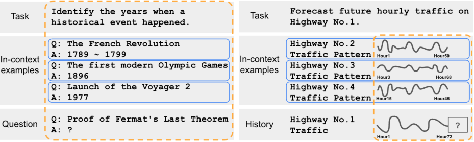
The Traditional Approach vs. In-Context Learning

Traditional time-series models see the world like this:

# Traditional approach (Prophet-style)
model = Prophet()
model.fit(historical_data)  # Training required
forecast = model.predict(future_dates)

# Traditional foundation model
forecast = timesfm.predict(
    historical_values[-512:]  # Only uses target series history
)

TimesFM-ICF introduces a paradigm shift:

# In-context fine-tuning approach
forecast = timesfm_icf.predict(
    target_history=web_traffic[-512:],
    context_examples=[
        competitor_traffic[-512:],      # Related series 1
        seasonal_pattern_last_year,      # Related series 2
        similar_product_launch_traffic,  # Related series 3
        # ... up to 50 examples
    ]
)

The Technical Architecture

The model architecture builds on the decoder-only Transformer design but with crucial modifications:

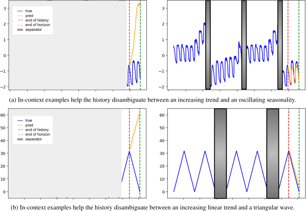
1. Separator Tokens: Special tokens delineate different time-series examples, preventing the model from interpreting concatenated series as a single continuous signal.
2. Cross-Example Attention: Unlike traditional architectures, the attention mechanism can look across different examples in the context window, learning patterns from related series.
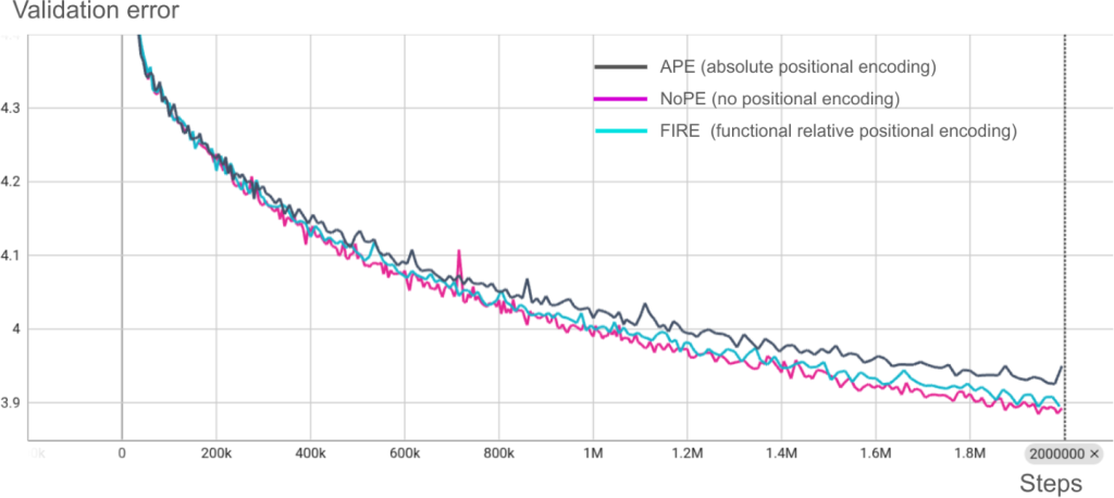
3. No Positional Encoding (NoPE): Counterintuitively, removing positional encodings improves length generalization – critical when context windows expand from 512 to 25,600 time points (50 examples × 512 points).
4. Patch-Based Processing: Each time-series is divided into patches (32 time points), embedded via residual blocks, and processed autoregressively.

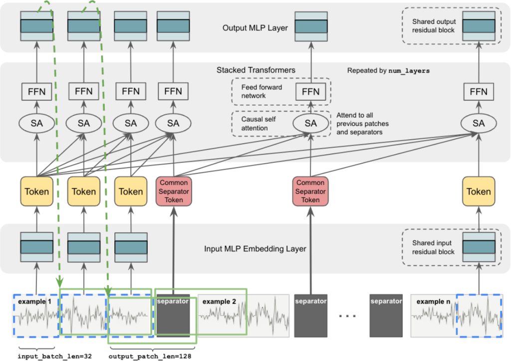
Here’s a simplified visualization of how data flows through the model:

[Series 1: E-commerce Site A Traffic]
    ↓ Patchify (32 points/patch)
[P1][P2][P3]...[P16][SEP]
         ↓
[Series 2: E-commerce Site B Traffic]  
[P1][P2][P3]...[P16][SEP]
         ↓
[Target Series: Your Site Traffic]
[P1][P2][P3]...[P12][PREDICT→][P13][P14][P15][P16]
         ↓
    Transformer with Cross-Example Attention
         ↓
    Future Predictions

Why This Matters: Solving Real Production Problems

Problem 1: Cold Start for New Products/Websites

Traditional Approach: Wait months to gather data, or use naive baselines.

Prophet-Style Solution:

# Not enough data for reliable seasonality detection
model = Prophet(yearly_seasonality=True)  # Guessing
model.fit(two_weeks_of_data)  # Unreliable

TimesFM-ICF Solution:

# Leverage similar product launches immediately
context_examples = [
    previous_product_launch_curves,
    category_average_patterns,
    seasonal_patterns_from_last_year
]
forecast = model.predict_with_context(new_product_data, context_examples)

Problem 2: Regime Changes and Black Swan Events

Traditional models struggle with sudden pattern changes. TimesFM-ICF can adapt in real-time by including recent examples of the new regime:

# COVID-19 traffic pattern shift example
pre_covid_patterns = traffic_jan_2020
early_covid_patterns = traffic_march_2020

# For April 2020 predictions, include March patterns as context
context = [
    early_covid_patterns,  # New regime examples
    similar_industry_covid_response,
    historical_crisis_patterns  # 2008 financial crisis
]

Problem 3: Multi-Resolution Forecasting

Unlike Prophet which requires separate models for different granularities, TimesFM-ICF handles multiple resolutions simultaneously:

# Single model, multiple granularities
hourly_context = [hourly_patterns_from_similar_days]
daily_context = [daily_patterns_from_similar_weeks]
weekly_context = [weekly_patterns_from_similar_quarters]

# Predict at any granularity using appropriate context
hourly_forecast = model.predict(target_hourly, hourly_context)
daily_forecast = model.predict(target_daily, daily_context)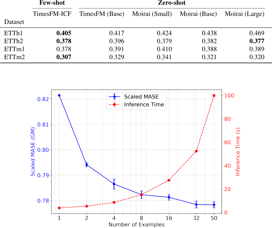

Practical Implementation Patterns

Pattern 1: The Context Library Approach

Build a library of canonical patterns for your domain:

class ContextLibrary:
    def __init__(self):
        self.patterns = {
            'black_friday': self.load_black_friday_patterns(),
            'product_launch': self.load_launch_patterns(),
            'seasonal_q4': self.load_q4_patterns(),
            'viral_growth': self.load_viral_patterns(),
            'paid_campaign': self.load_campaign_patterns()
        }

    def get_relevant_context(self, scenario_type, n_examples=10):
        """Retrieve relevant examples for current scenario"""
        base_patterns = self.patterns[scenario_type]

        # Add recency-weighted examples
        recent_similar = self.find_recent_similar_patterns()

        # Add diversity for robustness
        diverse_examples = self.sample_diverse_patterns()

        return base_patterns + recent_similar + diverse_examples

Pattern 2: Automated Context Selection

Use similarity metrics to automatically select relevant examples:

def select_context_examples(target_series, candidate_pool, n_examples=50):
    """
    Automatically select most relevant context examples
    using multiple similarity metrics
    """
    similarities = []

    for candidate in candidate_pool:
        # Statistical similarity
        dtw_distance = calculate_dtw(target_series[-100:], candidate[-100:])

        # Spectral similarity (frequency domain)
        spectral_sim = spectral_similarity(target_series, candidate)

        # Business metric similarity
        growth_rate_sim = compare_growth_rates(target_series, candidate)
        conversion_sim = compare_conversion_patterns(target_series, candidate)

        combined_score = weighted_average([
            dtw_distance, spectral_sim, growth_rate_sim, conversion_sim
        ])
        similarities.append((candidate, combined_score))

    # Return top N most similar
    return [s[0] for s in sorted(similarities, key=lambda x: x[1])[:n_examples]]

Pattern 3: Hierarchical Context Construction

For complex businesses with multiple levels of aggregation:

class HierarchicalContextBuilder:
    def build_context(self, target_store, target_category, target_sku):
        """
        Build context from multiple hierarchy levels
        """
        context = []

        # Company-wide patterns (macro trends)
        context.extend(self.get_company_patterns(n=5))

        # Store-level patterns (local effects)
        context.extend(self.get_similar_store_patterns(target_store, n=10))

        # Category patterns (product-type seasonality)
        context.extend(self.get_category_patterns(target_category, n=15))

        # SKU-level patterns (specific product behavior)
        context.extend(self.get_similar_sku_patterns(target_sku, n=20))

        return context[:50]  # Maximum 50 examples

Real-World Applications

1. E-commerce Conversion Rate Optimization

Instead of waiting weeks for A/B test results:

def predict_ab_test_outcome(test_config, early_results):
    """
    Predict full A/B test results from first 48 hours
    """
    context_examples = []

    # Historical tests with similar changes
    similar_tests = find_similar_ab_tests(test_config)
    context_examples.extend(similar_tests)

    # Seasonal patterns from same period last year
    seasonal = get_seasonal_patterns(test_config.start_date)
    context_examples.extend(seasonal)

    # Early adoption curves from similar features
    adoption_curves = get_feature_adoption_patterns(test_config.feature_type)
    context_examples.extend(adoption_curves)

    # Predict full test duration from early results
    predicted_outcome = timesfm_icf.predict(
        early_results,
        context_examples,
        horizon=test_config.duration_days * 24  # Hourly predictions
    )

    return predicted_outcome

2. Multi-Channel Marketing Attribution

Understanding channel interactions without complex MMM models:

def predict_channel_impact(channel_spend, other_channels_history):
    """
    Predict impact of channel spend changes using cross-channel patterns
    """
    # Include successful channel mix examples
    successful_campaigns = get_high_roi_campaign_patterns()

    # Include channel interaction patterns
    interaction_patterns = get_channel_interaction_examples()

    # Include competitive response patterns
    competitive_patterns = get_competitive_response_patterns()

    context = successful_campaigns + interaction_patterns + competitive_patterns

    return timesfm_icf.predict(
        target=channel_spend,
        context=context,
        output_metrics=['conversions', 'revenue', 'CAC']
    )

3. Real-Time Anomaly Detection with Context

Unlike traditional anomaly detection that relies on fixed thresholds:

class ContextualAnomalyDetector:
    def is_anomalous(self, current_pattern):
        """
        Determine if pattern is anomalous given context
        """
        # Get similar historical contexts
        similar_contexts = self.find_similar_contexts(current_pattern)

        # Predict expected pattern
        expected = timesfm_icf.predict(
            current_pattern[:-24],  # All but last 24 hours
            context=similar_contexts
        )

        # Calculate deviation
        actual = current_pattern[-24:]
        deviation = calculate_deviation(expected, actual)

        # Contextual threshold based on similar patterns' variance
        threshold = calculate_contextual_threshold(similar_contexts)

        return deviation > threshold

Performance Insights from the Paper

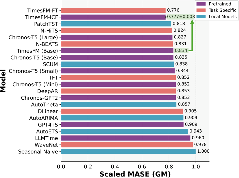
The empirical results are striking:

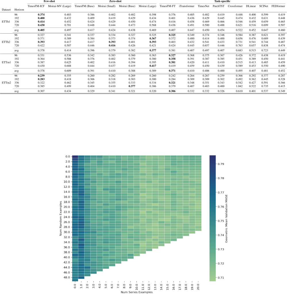
• 6.8% improvement over base TimesFM on out-of-domain benchmarks
• Matches fine-tuned model performance without any training
• 16x faster than traditional fine-tuning (25 minutes vs 418 minutes)
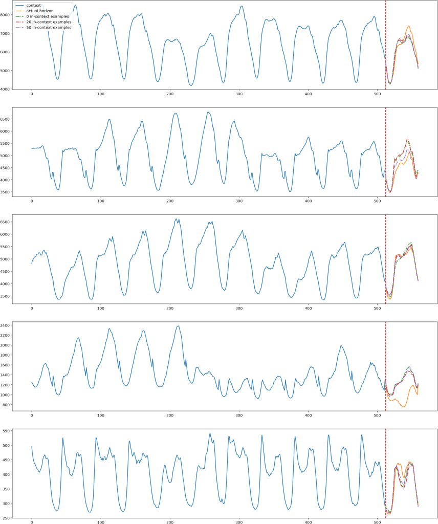
• Works with as few as 5 examples, scales up to 50

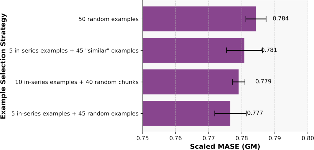
Most importantly, it shows that simple random selection of context examples often works well – you don’t need sophisticated retrieval mechanisms to start.

Migration Strategy: From Prophet to In-Context Learning

For teams currently using Prophet or similar tools, here’s a practical migration path:

Phase 1: Augment Prophet with Context

class ContextAugmentedProphet:
    def fit_predict(self, target_data, context_series_list):
        # Use Prophet for base forecast
        base_forecast = Prophet().fit(target_data).predict()

        # Use TimesFM-ICF for context-aware adjustment
        context_adjustment = timesfm_icf.predict(
            target_data,
            context_series_list
        )

        # Weighted combination
        return 0.7 * context_adjustment + 0.3 * base_forecast

Phase 2: A/B Test Against Current System

def compare_forecasting_approaches(historical_data):
    # Split data for backtesting
    train, test = temporal_train_test_split(historical_data)

    # Prophet baseline
    prophet_rmse = evaluate_prophet(train, test)

    # TimesFM-ICF with context
    context = select_similar_patterns(train)
    icf_rmse = evaluate_timesfm_icf(train, test, context)

    return {
        'prophet_rmse': prophet_rmse,
        'icf_rmse': icf_rmse,
        'improvement': (prophet_rmse - icf_rmse) / prophet_rmse
    }

Phase 3: Full Production Deployment

class ProductionForecastingService:
    def __init__(self):
        self.context_store = ContextStore()
        self.model = TimesFMICF()

    def forecast(self, series_id, horizon):
        # Get target series
        target = self.get_series(series_id)

        # Intelligently select context
        context = self.context_store.get_relevant_context(
            target,
            max_examples=50
        )

        # Generate forecast
        forecast = self.model.predict(target, context, horizon)

        # Add prediction intervals
        intervals = self.calculate_intervals(forecast, context)

        return {
            'forecast': forecast,
            'intervals': intervals,
            'context_used': context.metadata
        }

Future Implications and Opportunities

1. Federated Learning Without Training

Organizations can benefit from patterns across companies without sharing raw data:

# Company A provides encrypted pattern embeddings
company_a_patterns = encrypt_patterns(company_a_data)

# Company B uses these as context without seeing raw data
forecast = timesfm_icf.predict(
    company_b_data,
    context=[company_a_patterns, industry_benchmarks]
)

2. Real-Time Adaptation

Unlike traditional models that need retraining:

class AdaptiveForecaster:
    def predict_with_adaptation(self, target):
        # Morning prediction with overnight context
        morning_context = get_overnight_patterns()
        morning_forecast = predict(target, morning_context)

        # Afternoon update with morning actuals
        afternoon_context = morning_context + [morning_actuals]
        updated_forecast = predict(target, afternoon_context)

        return updated_forecast  # No retraining needed

3. Cross-Domain Transfer

Apply patterns from completely different domains:

# Use viral social media patterns to predict product adoption
social_viral_patterns = get_tiktok_viral_patterns()
product_forecast = predict(
    new_product_sales,
    context=[social_viral_patterns, previous_product_launches]
)

A New Era for Time-Series Forecasting

TimesFM-ICF represents more than an incremental improvement – it’s a fundamental shift in how we approach time-series forecasting. By borrowing the in-context learning paradigm from LLMs, it offers:

• Immediate deployment for new products/scenarios
• No training infrastructure required
• Dynamic adaptation to changing patterns
• Cross-domain learning opportunities

For practitioners, this means less time managing model pipelines and more time understanding business context. The question isn’t whether to adopt in-context forecasting, but how quickly you can build your context library and migration plan.

The age of “train once, deploy everywhere” forecasting has arrived. The only question is: what patterns will you discover when you can learn from any related time-series, anywhere, instantly?

---

Based on the paper and current information available, here’s the status of model availability:

Keep in Mind

• Not yet publicly available – The paper was just presented at ICML 2025
• No GitHub repository currently available for TimesFM-ICF specifically
• No Vertex AI deployment announced yet

TimesFM (Base model – without in-context learning)

The original TimesFM that this work builds on is available:

GitHub Repository: https://github.com/google-research/timesfm

Hugging Face:

• Model: https://huggingface.co/google/timesfm-1.0-200m
• PyPI Package: pip install timesfm

Current Usage Example (Base TimesFM):

import timesfm

tfm = timesfm.TimesFm(
    context_len=128,
    horizon_len=24,
    input_patch_len=32,
    output_patch_len=128,
    num_layers=20,
    model_dims=1280,
    backend='cpu'  # or 'gpu'
)
tfm.load_from_checkpoint(repo_id="google/timesfm-1.0-200m")

forecast = tfm.forecast(
    time_series_data,
    freq="D"  # Daily frequency
)

Alternative Approaches

Consider these available alternatives that offer some similar capabilities:

MOMENT (Multi-variate forecasting):
pip install momentfm
https://github.com/moment-timeseries-foundation-model/moment

Chronos (Amazon’s foundation model):
pip install chronos-forecasting
https://github.com/amazon-science/chronos-forecasting

Lag-Llama (probabilistic forecasting):
https://github.com/time-series-foundation-models/lag-llama

Expected Timeline

The authors’ email addresses from the paper (senrajat@google.com, abhidas@google.com) suggest they’re at Google Research, so the model will likely follow Google’s standard productization path through Vertex AI eventually.

I’ll update the article when the model becomes publicly available. For now, the base TimesFM offers solid zero-shot capabilities, just without the powerful in-context learning feature that makes ICF special.