Semantic Similarity Rating (SSR) maps LLM free-text responses to Likert distributions to improve purchase intent realism and match human response patterns.
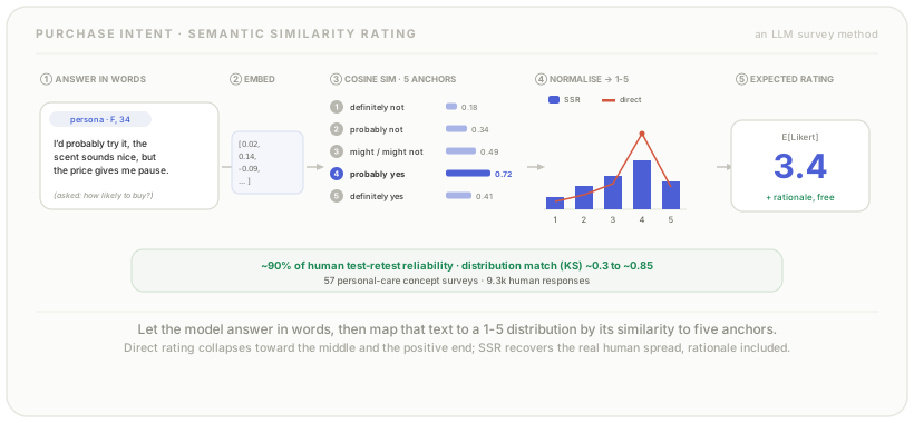
Instead of forcing LLMs to pick a number on a 1–5 scale, ask them to speak like a person and map the text to a Likert distribution via Semantic Similarity Rating (SSR). In benchmarks across 57 personal-care concept surveys (9.3k human responses), SSR reproduced human purchase intent signals with ~90% of human test–retest reliability and much closer response distributions than direct Likert elicitation. Plus, you get qualitative rationale for free.
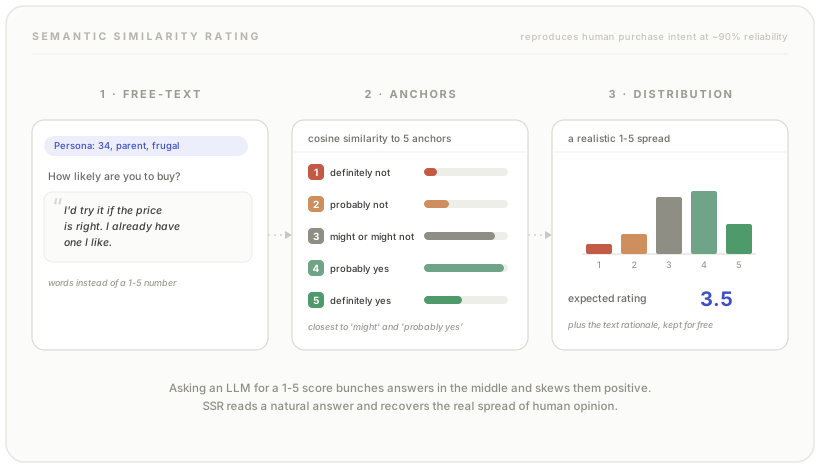
Why you should care
- Directly asking an LLM for 1..5 tends to collapse into the middle (regression to mean) and over-positivity. Distributions end up unrealistic.
- SSR fixes this by: (1) eliciting a short free-text PI statement; (2) embedding it; (3) computing cosine similarity to five anchor statements (one per Likert level) and normalising into a probability mass function across 1–5.
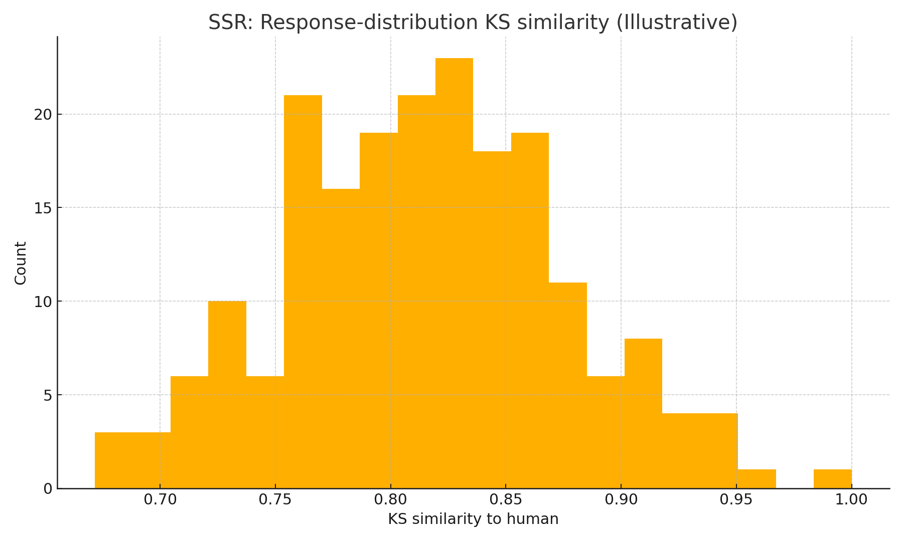
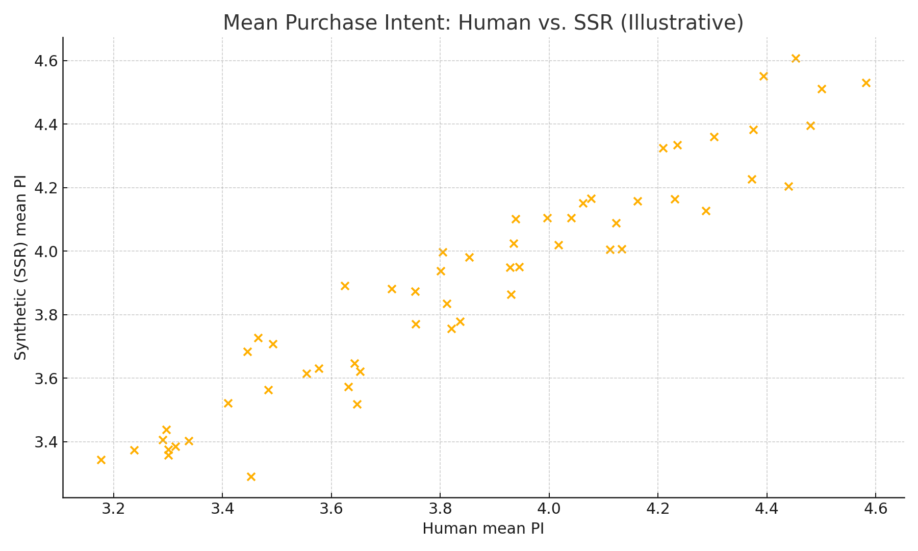
- On 57 real surveys, SSR closed the realism gap: distribution similarity (KS) jumped to ≈0.8–0.9, while correlation of mean PI vs. humans improved or matched FLR.
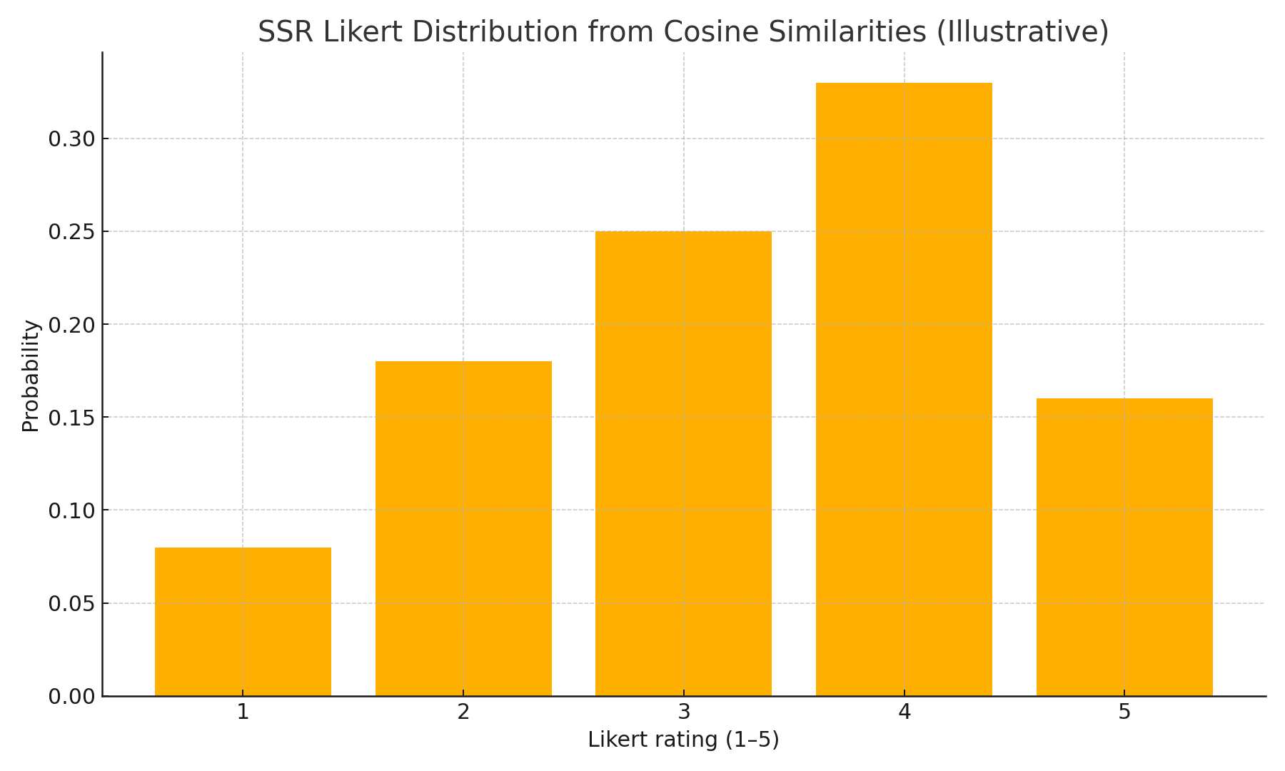
Method in one picture
- Prompt the model to impersonate a respondent with demographics; show the concept; ask “How likely are you to buy?” but allow short free-text.
- Embed the text and compare to five anchors (Likert 1–5).
- Normalise cosine similarities to a pmf over 1..5, then compute the expected rating.
What the paper found (and what to expect)
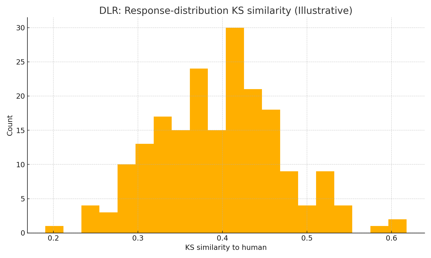
- DLR (Direct Likert Rating): OK correlation (~0.8 ρ attainment) but poor distribution match (KS ≈ 0.26–0.45 depending on model/temperature).
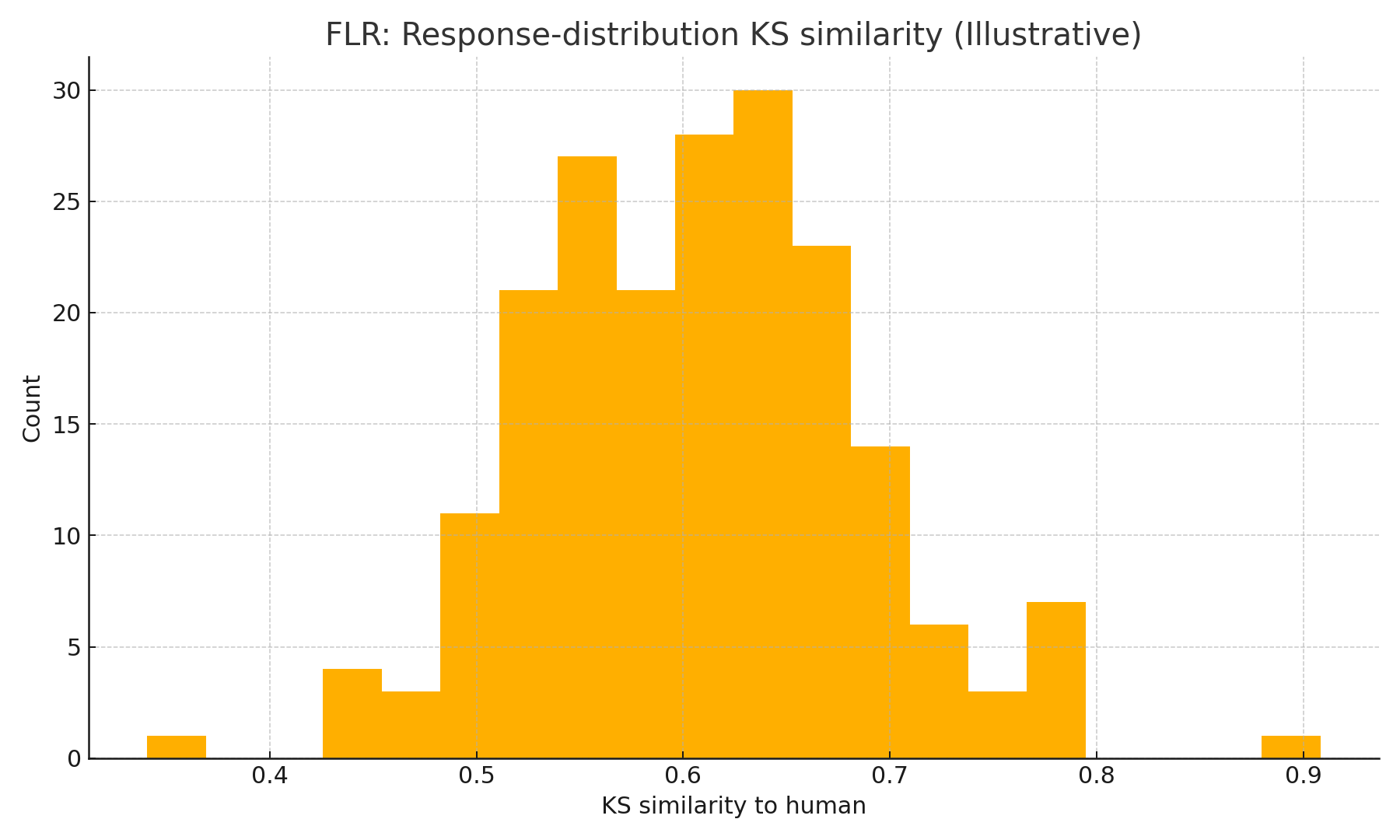
- FLR (Follow-up Likert after text): higher KS than DLR; solid correlation; needs a good “Likert-expert” rater prompt.
- SSR (this article): best distributional realism (KS ≥ ~0.8) and mean-PI correlation on par with (or better than) FLR.
Illustrative histograms below show the direction of change (not the study data):
Implementation choices that matter
- Anchors: Use 5 concise, domain-agnostic statements (from “definitely not” → “definitely yes”); average over multiple anchor sets to stabilise.
- Embeddings model: The paper used OpenAI embeddings; with Google’s Gemini API you can use
gemini-embedding-001 and the new GenAI SDK’s models.embed_content. - Persona: Adding demographic attributes to the generator improves signal; without it, correlation drops even if distributions look realistic.
Minimal SSR recipe
- Generate a short, natural PI statement with
gemini-2.5-flash. - Embed: compute vectors for the statement and five anchors with
gemini-embedding-001 via client.models.embed_content(...). - Score: cosine similarity → normalise → pmf → expected Likert (E[Likert]).
- Report: show the pmf, the expected score, and the text rationale.
An illustrative correlation-style scatter (not study data):
Practical notes
- Keep anchors short/generic; don’t bake in product features.
- Use 2–6 anchor sets and average pmfs.
- For reproducibility, set model temperature low for generation, e.g. 0.2–0.5 (the paper shows little sensitivity to temperature overall).
- Track both ranking signal (correlation of mean PI) and distribution similarity (e.g., KS).
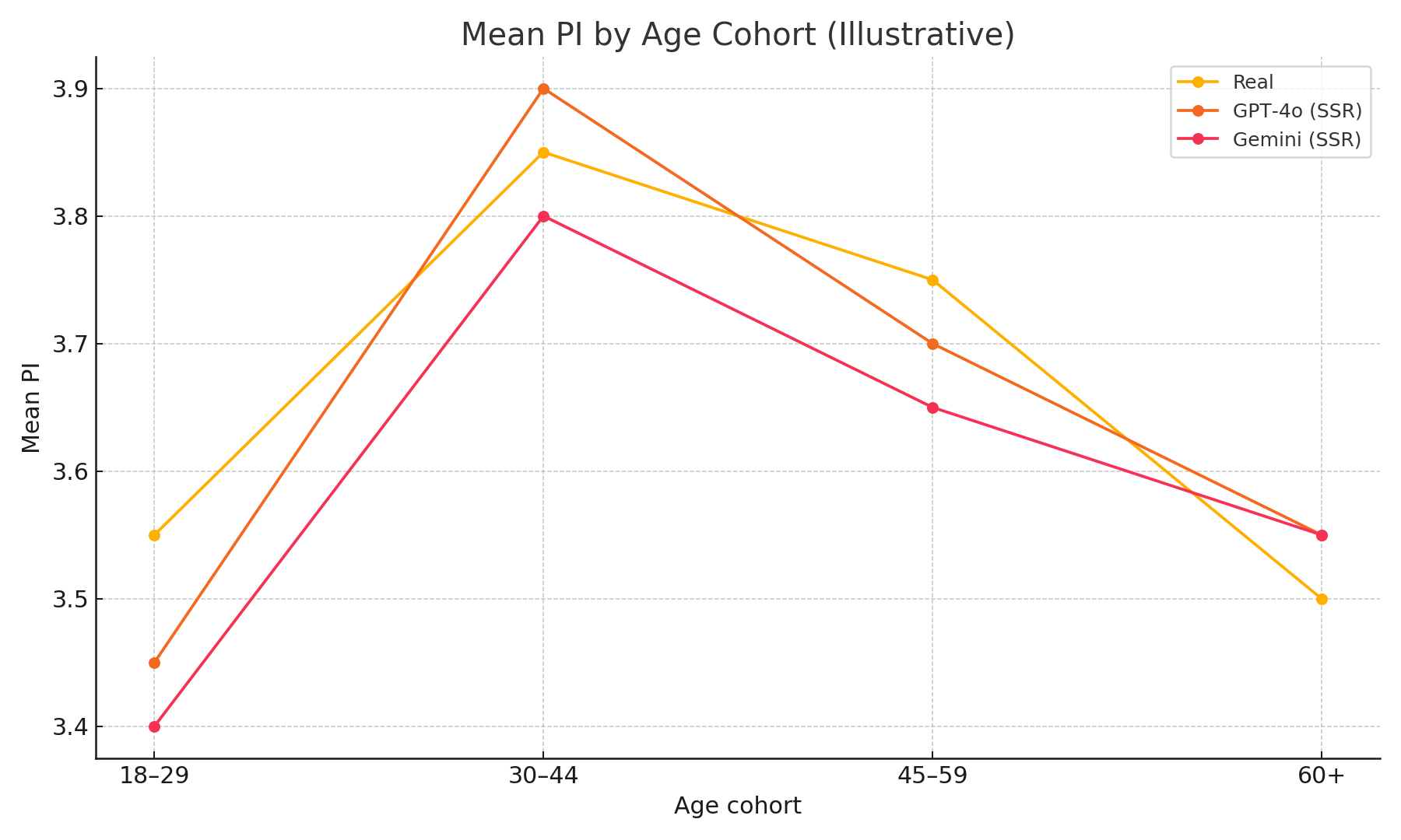
A stylised demographic slice (not study data):
Assets included (use in your post)
fig1_ssr_mapping.png — Likert pmf produced by SSR (illustrative).fig2_dlr_ks_hist.png — DLR KS histogram (illustrative).fig2b_flr_ks_hist.png — FLR KS histogram (illustrative).fig2c_ssr_ks_hist.png — SSR KS histogram (illustrative).fig3_correlation_scatter.png — Human vs. SSR mean PI (illustrative).fig4_demographic_stratified.png — Mean PI by age cohort (illustrative).
Keep in mind
- Anchor selection can bias the mapping; average across sets and document anchor text.
- Distributions may look “too good” without personas while losing ranking signal; don’t drop demographics blindly.
- Respect privacy & brand IP when using real concepts; follow Google’s prohibited-use policies for the API.
References
- Maier, B. F. et al. LLMs Reproduce Human Purchase Intent via Semantic Similarity Elicitation of Likert Ratings, 2025.
- Gemini 2.5 Flash & model IDs:
gemini-2.5-flash. - Embeddings via GenAI SDK:
models.embed_content with gemini-embedding-001.
Paper:
2510.08338v2 – LLMs Reproduce Human Purchase Intent via Semantic Similarity Elicitation of Likert RatingsDownload

 Dan Petrovic ·
15 October 2025
Dan Petrovic ·
15 October 2025