An evaluation of Explorative Modeling on a text diffusion model: a small consistent gain at matched steps, and a larger likelihood-versus-sampling tradeoff that turned out to belong to the training schedule.
The corpus is 579,508 documents, 1.81 billion characters, deduplicated, with 4,000 documents held out for validation and 4,000 for test. The tokenizer is a 32,768-token byte-level BPE trained on the training split. Tokenized, training data comes to 390.3M tokens at 4.57 characters per token.
The model is a 115.7M-parameter masked diffusion language model — 12 layers, 12 heads, d_model 768, SwiGLU feed-forward, RoPE, shared adaLN — trained from random initialisation with continuous-time absorbing-state MDLM (Sahoo et al. 2024) on a linear schedule.
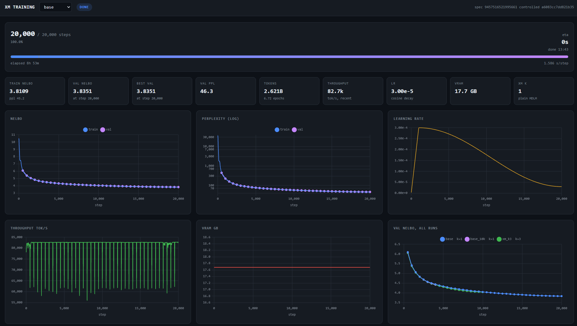
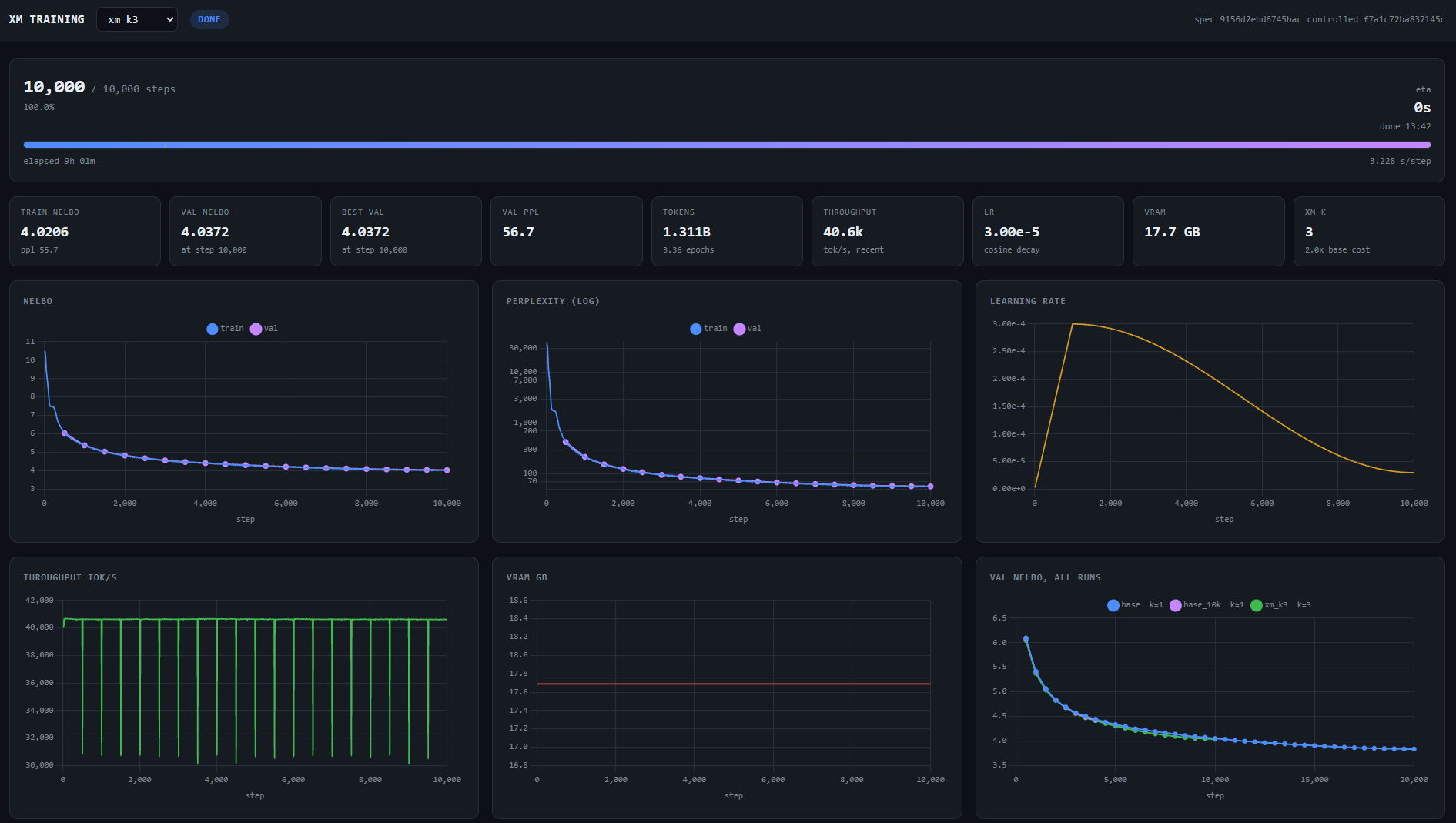
We trained it twice on one RTX 4090: a plain baseline for 20,000 steps in 8h 53m, and XM at K=3 for 10,000 steps in 9h 01m. XM costs 2x per step, so those are the same compute, and that is the pairing.
Both arms were evaluated on test-set likelihood and on generative perplexity across sampling budgets from 8 denoising steps up to 256, scored by a frozen external model. The two measurements point different ways.
Update, 4 August 2026. The base_10k control referred to throughout this post has since finished, and it overturns part of what is written below. The likelihood deficit was run length, not XM, and about three quarters of the 15.2% sampling gain was run length too. The original text is left unedited; the corrected numbers are in UPDATE: the base_10k control at the end.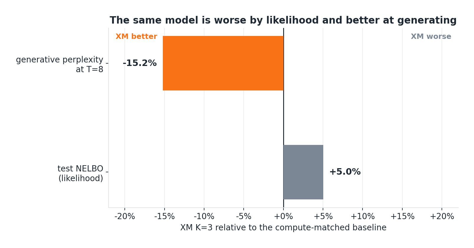
The rest of this post is the breakdown, one result we did not expect, and what we have not finished checking.
| architecture | 12L / 12H / d_model 768 / d_ff 2048 (SwiGLU), RoPE, shared adaLN |
| params | 115.7M total, 90.5M non-embedding |
| objective | continuous-time absorbing-state MDLM (Sahoo et al. 2024), linear schedule |
| vocab | 32,768 byte-level BPE, trained on the train split only |
| corpus | 390.3M train tokens, 4.57 chars/token |
| seq len | 512 |
| batch | 32 x 8 accum = 256 seqs = 131,072 tokens/step |
| hardware | one RTX 4090, bf16, no torch.compile |
Two arms, matched on wall-clock rather than on steps:
| run | K | steps | tokens | epochs | wall |
|---|---|---|---|---|---|
base |
1 | 20,000 | 2.62B | 6.72 | 8h 53m |
xm_k3 |
3 | 10,000 | 1.31B | 3.36 | 9h 01m |
XM at K=3 costs (K+3)/3 = 2.0 baseline steps: K forward passes under no_grad to score the candidates, then a full forward and backward for the winner, against a baseline step of one forward plus one backward. Measured: 3.25 s/step vs 1.60, a ratio of 2.03x against the predicted 2.00x. So 10,000 XM steps and 20,000 baseline steps are the same spend, and that is the pairing.
Peak VRAM was 17.7 GB for both arms, identical to the digit. Recomputing the winner rather than retaining K graphs (--xm-chunk 1, the reference's save_mem_mode) fully absorbs the exploration cost. XM is free in memory and 2x in time.
The reference NLP branch selects one of K embeddings appended past the vocab and prepends it as an extra sequence position. We instead add it to the timestep conditioning vector that feeds adaLN. The reason is that prepending takes the sequence from 512 to 513 and shifts every RoPE position relative to the baseline, which would confound the comparison; adding to c leaves the architecture byte-identical between arms, so --xm-k is the only difference.
We do not know whether this matters. It is the first thing we would ask the authors about.
We also evaluate all K latents for every sample rather than drawing random candidates per chunk, which makes the selection an exact argmin rather than a K-sample estimate of one. Lower variance, and K is small enough that there is no reason to sample.
| test NELBO | ppl bound | |
|---|---|---|
base @ 20,000 |
3.844 | 46.70 |
xm_k3 @ 10,000 |
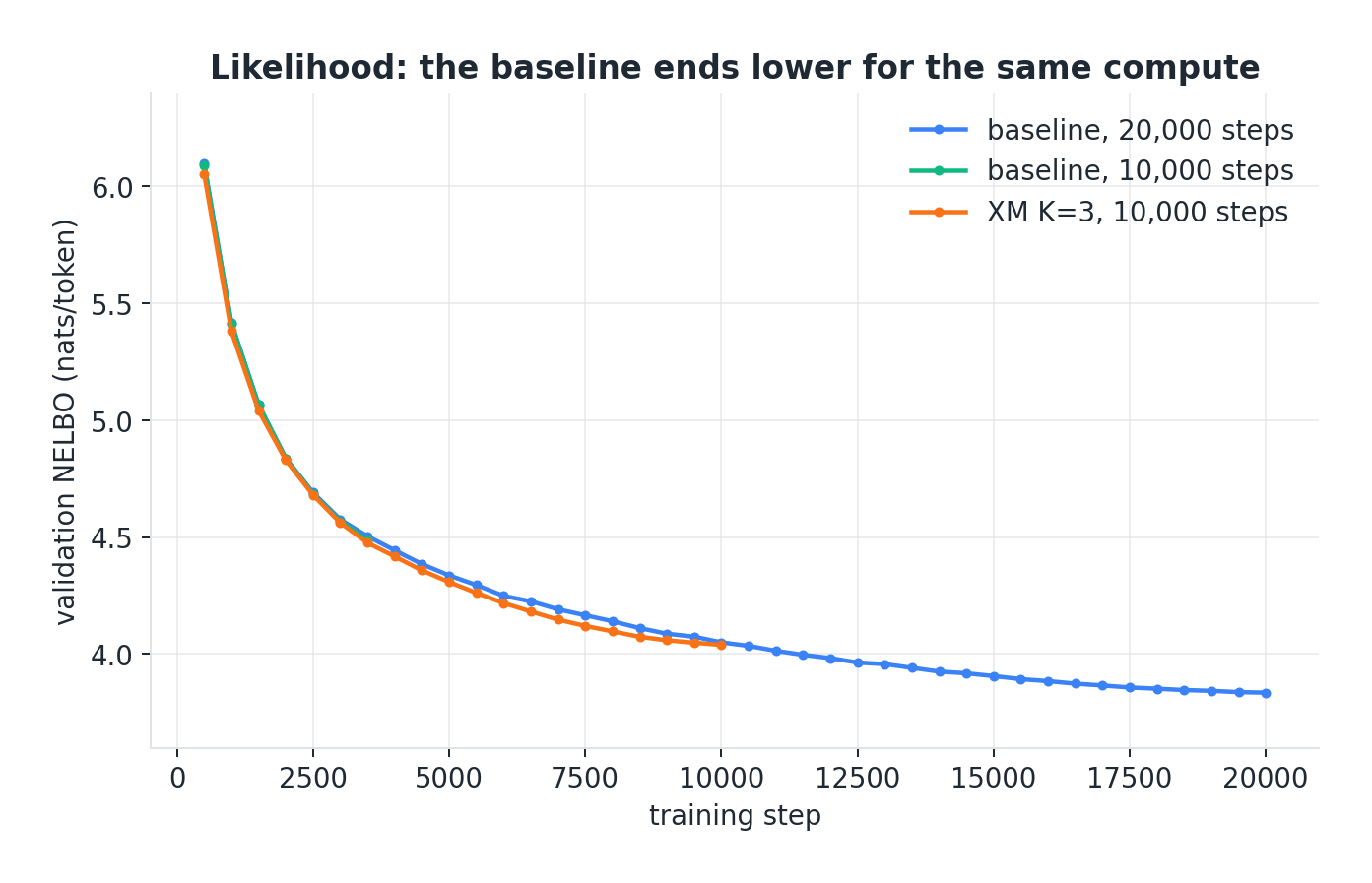
4.037 | 56.68 |
0.19 nats, same nine hours. Not marginal.
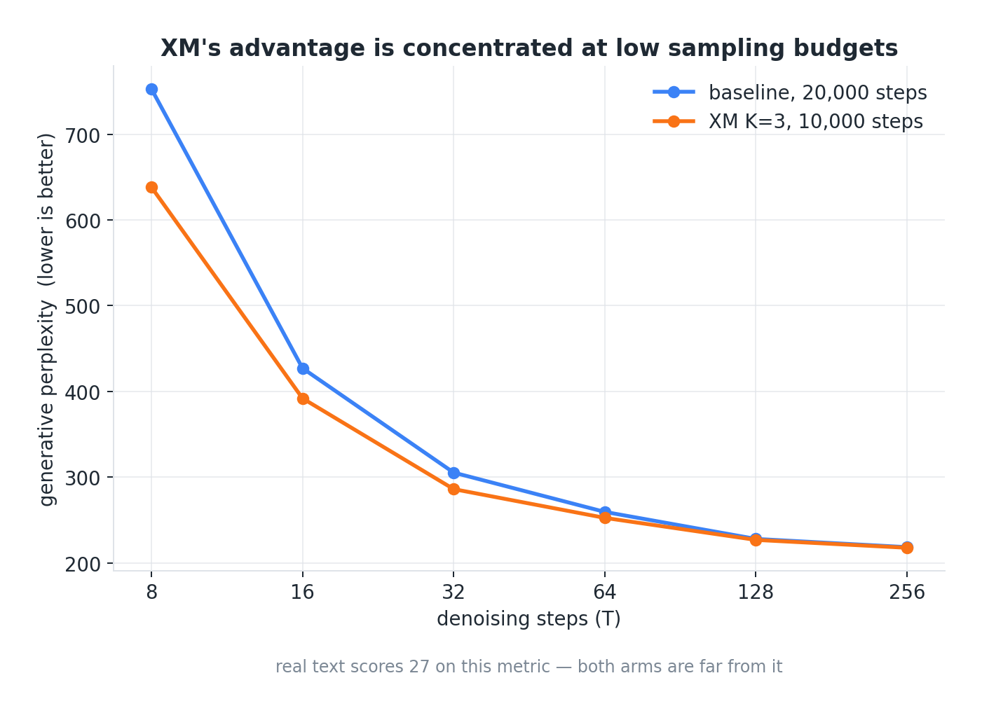
Generative perplexity under a frozen scorer (gemma-3-270m, revision 9b0cfec8), 1024 samples per setting, 256 tokens each, temperature 1.0, no top-p or top-k, seed 1337.
| T | base |
xm_k3 |
delta |
|---|---|---|---|
| 8 | 752.9 | 638.3 | -15.2% |
| 16 | 427.1 | 392.0 | -8.2% |
| 32 | 305.4 | 286.1 | -6.3% |
| 64 | 259.5 | 252.5 | -2.7% |
| 128 | 228.0 | 226.8 | -0.5% |
| 256 | 218.4 | 217.7 | -0.3% |
| real text | 27.0 | 27.0 |
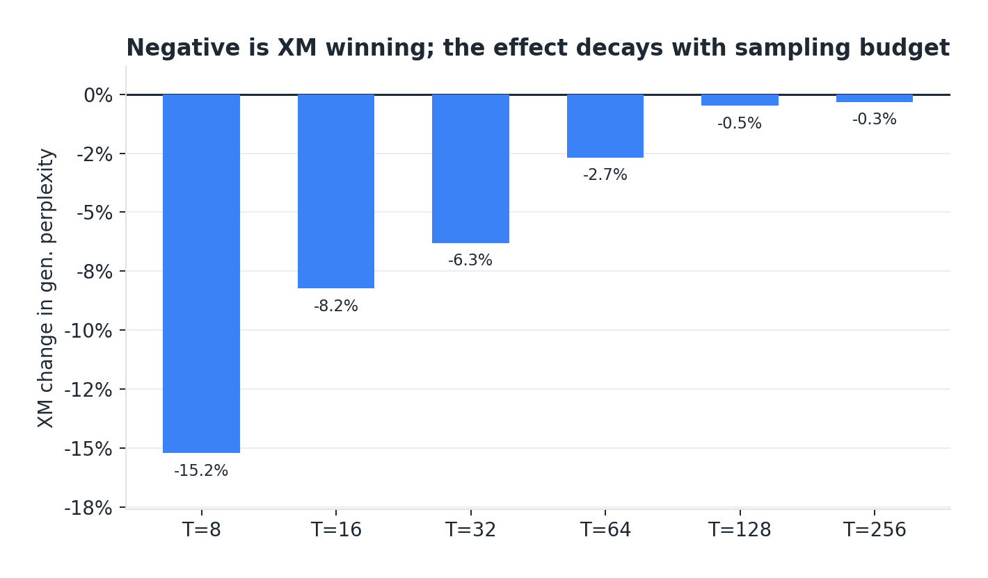
Six settings, monotone ordering, largest effect where the sampler has the least budget. Noise does not sort itself into a monotone sequence across six independent settings, so we believe the effect is real — but see the pending list, we do not yet have confidence intervals on it.
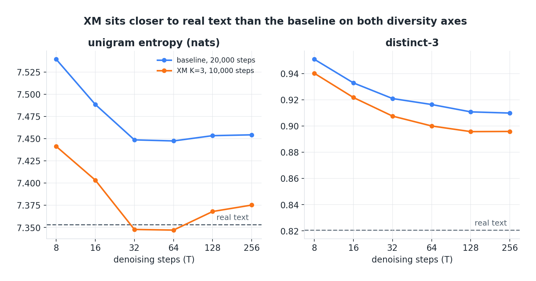
It is not bought by narrowing. The usual way to fake a generative perplexity win is to collapse toward high-probability text. Both models are in fact too diverse relative to real text, and XM is less so on both axes:
| T=8 | entropy (nats) | distinct-3 |
|---|---|---|
base |
7.539 | 0.951 |
xm_k3 |
7.441 | 0.940 |
| real text | 7.353 | 0.821 |
XM moves toward the data on both while also improving perplexity. The entropy gap of 0.098 nats is roughly 3x our measurement floor at 1024 samples (+/- 0.03), so unlike smaller runs we have looked at, this one is actually resolvable.
As a sampling-efficiency claim, it is more modest than 15% sounds. Interpolating the baseline curve to find where it matches XM's quality:
xm_k3 @ T=8   equals base @ T ~ 9.8    1.2x fewer sampling steps
xm_k3 @ T=16  equals base @ T ~ 19.1   1.2x fewer sampling steps
The curve is steep at low T, so a 15% perplexity gain converts to about 1.2x in steps. Inference cost per step is identical between the arms — generation samples one latent and runs one forward — so that 1.2x is a real deployment saving, paid for with 2x training compute.
The intuitive story for XM is that the K latents specialise into distinct modes, and best-of-K training lets each document be explained by whichever mode fits it.
That is not what happened. The latents are redundant.
Read that second number again. We let the model look at the true loss and pick whichever of its three latents scored best on that specific sample, and the oracle peek bought two thousandths of a nat. The three latents converged to nearly identical predictive distributions.
And XM improved low-step sampling anyway.
So whatever the mechanism is, it does not appear to be mode specialisation. Our current guess is that it is a training-dynamics effect rather than a representational one — the argmin acts as a per-sample loss filter, and the gradient the model receives is systematically the easier of three draws. That would be a curriculum effect, not a mixture effect, and it would explain why the benefit shows up in sampling robustness rather than in likelihood. We have not tested this.
If someone has a better hypothesis, we would like to hear it.
wmax — the largest per-latent share of argmin wins over a logging window — reads like total collapse for the first ~50 steps of every XM run, then breaks symmetry, relapses, and breaks again:
step  10   0.935 / 0.029 / 0.036
step  20   0.995 / 0.004 / 0.002
step  30   0.998 / 0.002 / 0.001
step  40   0.997 / 0.003 / 0.000
step  50   0.984 / 0.009 / 0.007
step  60   0.486 / 0.341 / 0.173     <- symmetry breaks here
step  80   0.750 / 0.131 / 0.119     <- and partially relapses
step 110   0.889 / 0.045 / 0.065
step 140   0.443 / 0.299 / 0.258
step 200   0.429 / 0.269 / 0.302
...
step 10000 0.361 / 0.347 / 0.292
The cause is adaLN-zero initialisation. At step 0 the conditioning vector has no effect on the output, so all K latents score identically and argmin returns index 0 for every sample. Losing latents receive no gradient at all in our setup (the latent rows live in reserved vocab slots that are forced to -inf in the logits, so they train only through cond), which looks like a permanent dead-unit trap on paper. It isn't. Once adaLN leaves zero the winner's embedding moves, conditioning starts to matter, and the untouched rows become competitive on a subset of samples.
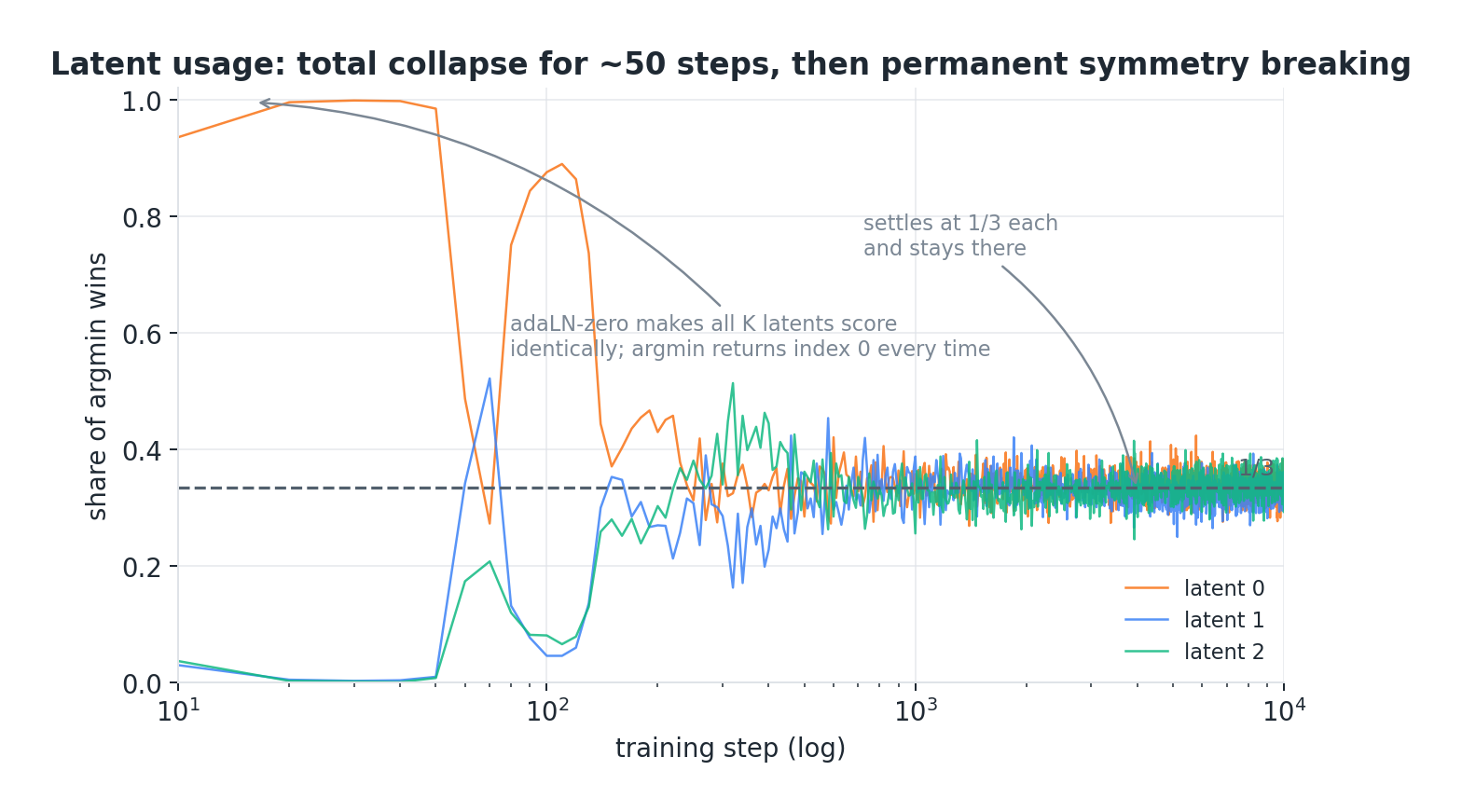
Practical consequence: do not smoke-test XM for 30 steps and conclude your implementation is broken. The transient runs to roughly step 150 and is not monotone. Read wmax after step 200.
We are publishing this early because the dissociation is worth talking about, not because it is finished. Open, in order of how much they could change the story:
base ran 20,000 steps, xm_k3 ran 10,000. Both completed their own cosine schedule, so both are fully annealed — but we cannot yet rule out that a fully-annealed 10,000-step model simply samples better at low T than a fully-annealed 20,000-step one, for reasons unrelated to XM. A base_10k control sharing xm_k3's exact schedule is running as we write this, and we will append the result. If it beats base at T=8, this post's headline belongs to the learning rate schedule and not to XM.base shrinks substantially when compared against a 10,000-step baseline instead of a 20,000-step one.Numbers, configs and the exact spec hashes for both runs are reproducible from the run directories; every run logs a controlled_hash covering everything the two arms are required to share, so the comparison is machine-checkable rather than asserted.
More on XM: https://explorative-modeling.github.io/
Appending base_10k when it completes training.
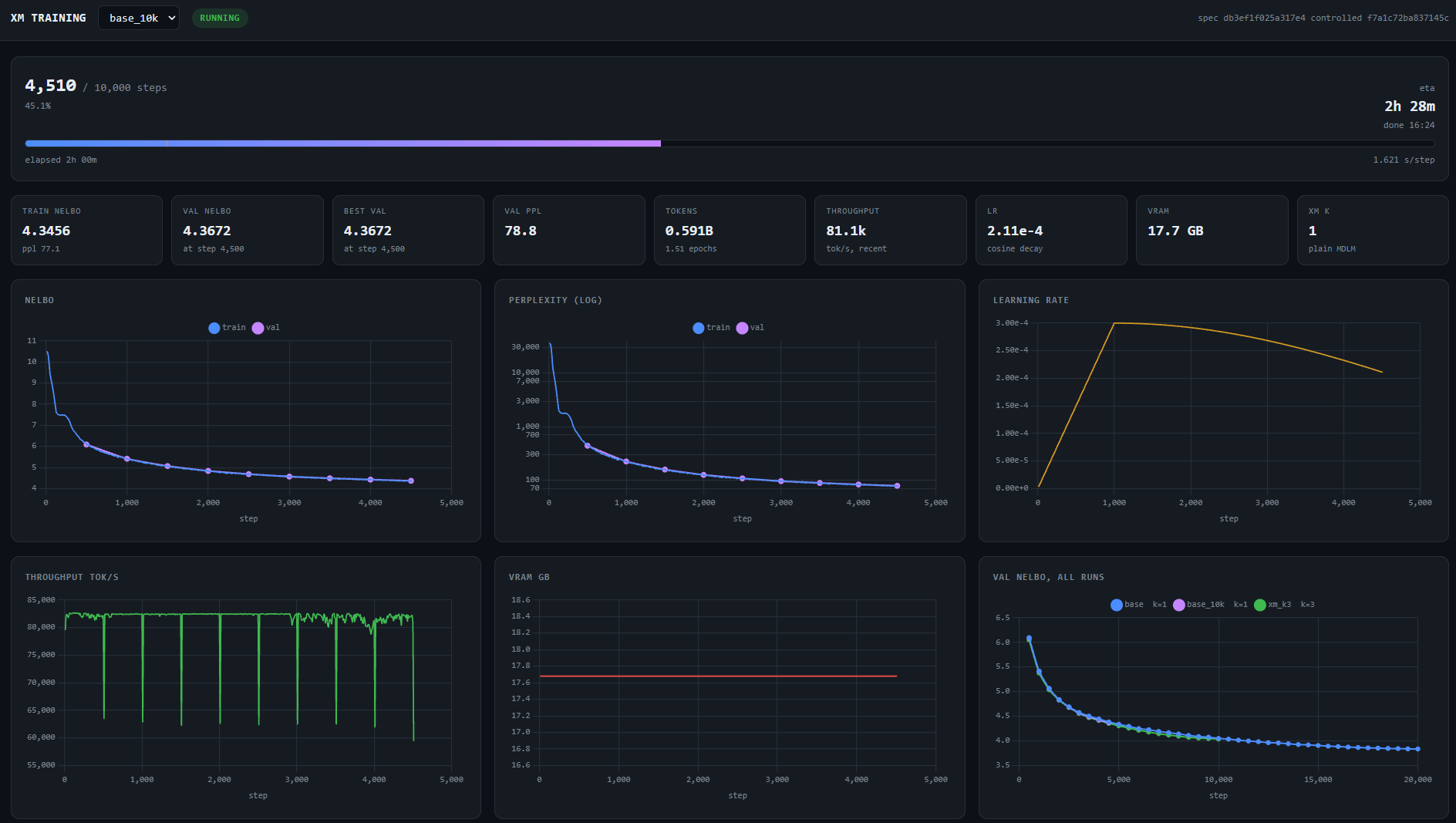
base_10k control, and what it does to the result abovebase_10k finished. It is a plain MDLM baseline on xm_k3's exact schedule — 10,000 steps, same cosine anneal, same seed, same everything but --xm-k. Both runs report controlled f7a1c72ba837145c, so the comparison needs no exemption flag. It took 4h 27m at 1.603 s/step against xm_k3's 9h 01m at 3.228, which confirms the 2x cost model a third time.
It changes the conclusion. Most of what this post attributed to XM belongs to run length.
| run | K | steps | wall | test NELBO | ppl bound |
|---|---|---|---|---|---|
base |
1 | 20,000 | 8h 53m | 3.8438 | 46.70 |
xm_k3 |
3 | 10,000 | 9h 01m | 4.0374 | 56.68 |
base_10k |
1 | 10,000 | 4h 27m | 4.0470 | 57.22 |
| T | base 20k |
base_10k |
xm_k3 |
|---|---|---|---|
| 8 | 752.9 | 669.4 | 638.3 |
| 16 | 427.1 | 405.0 | 392.0 |
| 32 | 305.4 | 289.3 | 286.1 |
| 64 | 259.5 | 253.6 | 252.5 |
| 128 | 228.0 | 232.4 | 226.9 |
| 256 | 218.4 | 220.8 | 217.7 |
| real text | 27.0 | 27.0 | 27.0 |
At matched steps XM is ahead: 4.0374 against 4.0470, a margin of 0.010 nats. The 0.19-nat deficit in the body of this post is the gap between 10,000 steps and 20,000 steps. It is not a property of XM, and the title of this post is wrong about it.
Against the equal-steps control, XM's T=8 gain is -4.6%, not -15.2%.
| T=8 delta | |
|---|---|
base_10k vs base @ 20k (run length) |
-11.1% |
xm_k3 vs base_10k (XM) |
-4.6% |
xm_k3 vs base @ 20k (both, as published) |
-15.2% |
Roughly three quarters of the headline number is the schedule. Halving a baseline's training improves its low-step generative perplexity by 11% on its own, at half the compute.
The run-length effect is specific to a starved sampler and reverses once the sampler has budget: base_10k is 11.1% better than base at T=8 and 1.1% worse at T=256.
The body of this post argued the XM win was not bought by narrowing, on the grounds that XM sat at 7.441 nats against the baseline's 7.539, closer to real text's 7.353. base_10k sits at 7.438 — the same place. The diversity shift came from training less, not from XM.
At matched steps there is no diversity difference to speak of:
| T=8 | entropy (nats) | distinct-3 |
|---|---|---|
base @ 20k |
7.539 | 0.951 |
base_10k |
7.438 | 0.940 |
xm_k3 |
7.441 | 0.940 |
| real text | 7.353 | 0.821 |
XM's entropy edge over base_10k is +0.003 nats at T=8 and within +/-0.03 — our measurement floor at 1024 samples — at all six settings. distinct-3 is identical to three decimals.
A strict frontier win, smaller than advertised and cleaner than advertised. xm_k3 beats base_10k at every one of the six sampling budgets, and pays nothing in diversity to do it. Against base @ 20,000 the gain came with 0.098 nats of entropy given up; against the matched control it comes with none.
As a sampling-efficiency claim it is thin. Interpolating the base_10k curve, xm_k3 at T=8 matches it at T ~ 8.5 — about 1.07x fewer sampling steps, for 2x the training compute.
The finding this post was built around — likelihood and low-step sample quality moving in opposite directions — holds up. It just belongs to the training schedule. base_10k against base @ 20,000 is 0.20 nats worse on the test NELBO and 11.1% better at T=8, with nothing varying but the number of steps.
More training buys likelihood and costs you the truncated sampler. We did not set out to measure that and have no explanation for it. It is the larger of the two effects here by a factor of two and a half.
Everything in the pending list above except item 2, which this appendix closes. One seed per arm, no confidence intervals, one scale, one K, and absolute quality still bad enough that all three models produce text nobody would read. The latent redundancy result is unchanged — usage 0.33/0.33/0.33, best-of-3 worth 0.002 nats over the mixture bound — and now has to explain a 4.6% effect rather than a 15.2% one.
 Dan Petrovic ·
04 August 2026
Dan Petrovic ·
04 August 2026